SquareNet

❒ SquareNet — Bijective Gridification of Point Clouds

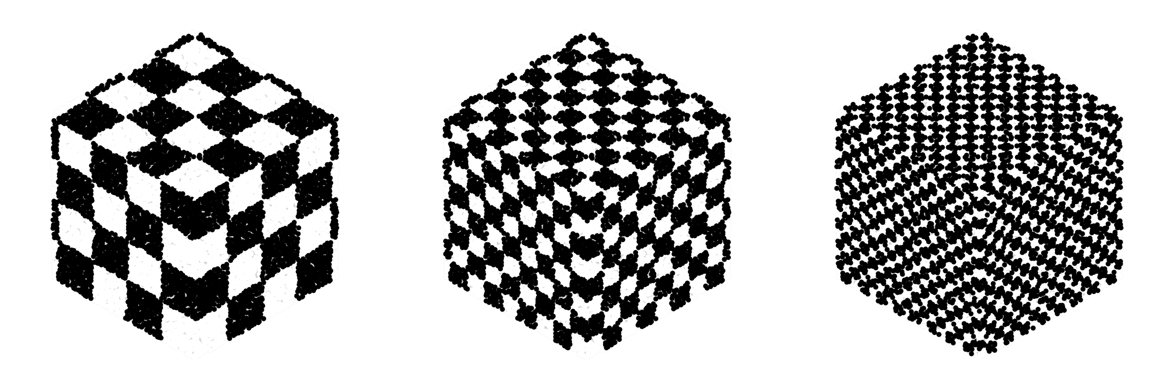
SquareNet maps unstructured point clouds to structured grids through a bijective transformation: one point, one cell, no overlap, fully invertible ¹.

The practical payoff: you replace expensive spatial queries (k-NN, radius search, neighborhood graphs) with plain tensor indexing. Think of it as an alternative to kd-trees, voxelization, rasterization, or graph-based approaches, but with a regular tensor structure allowing for massive parallelisation.

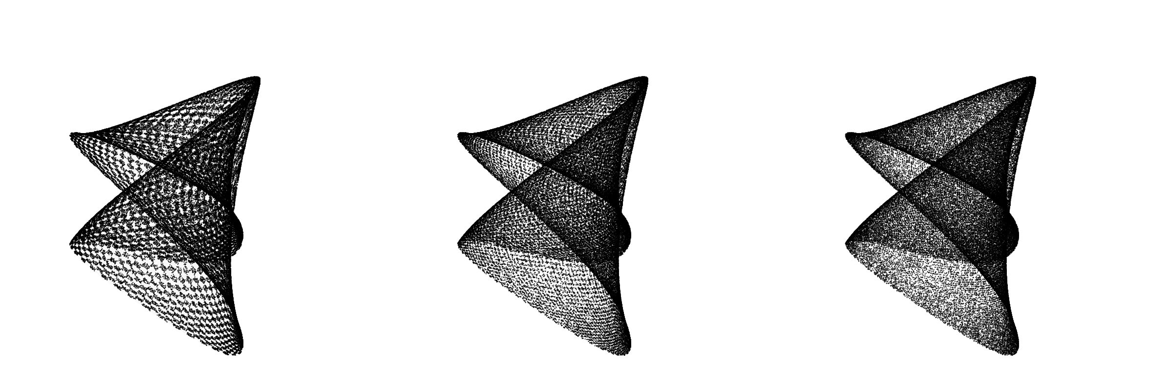
✔ Works in any dimension
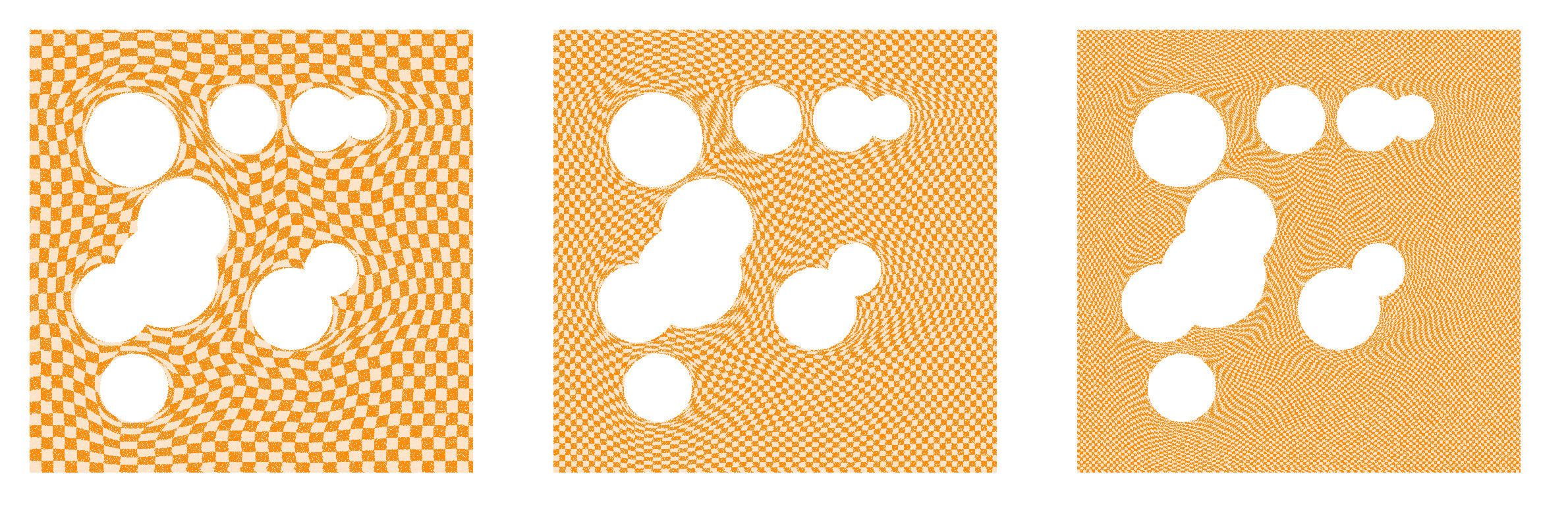
✔ Handles non-convex geometries and irregular distributions
✔ Scales to millions of points (seconds, not minutes)
✔ Compatible with PyTorch and JAX

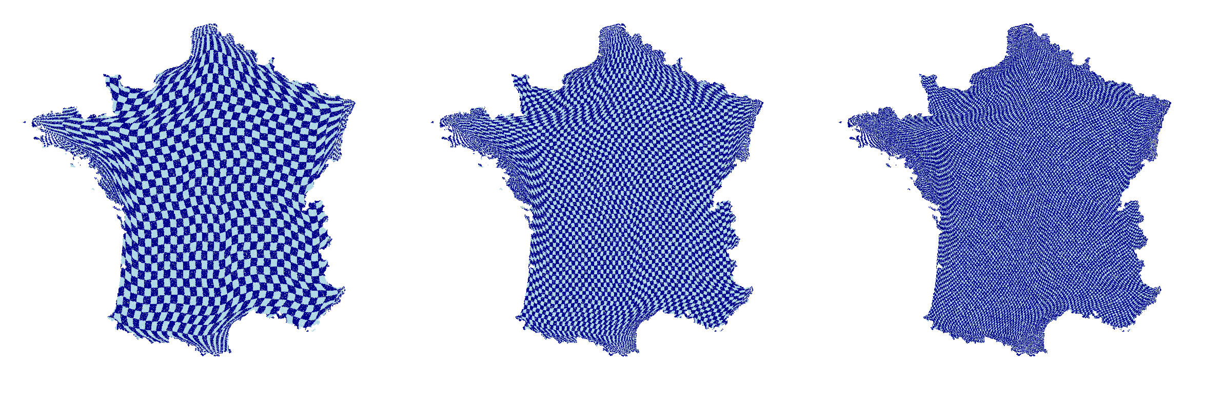
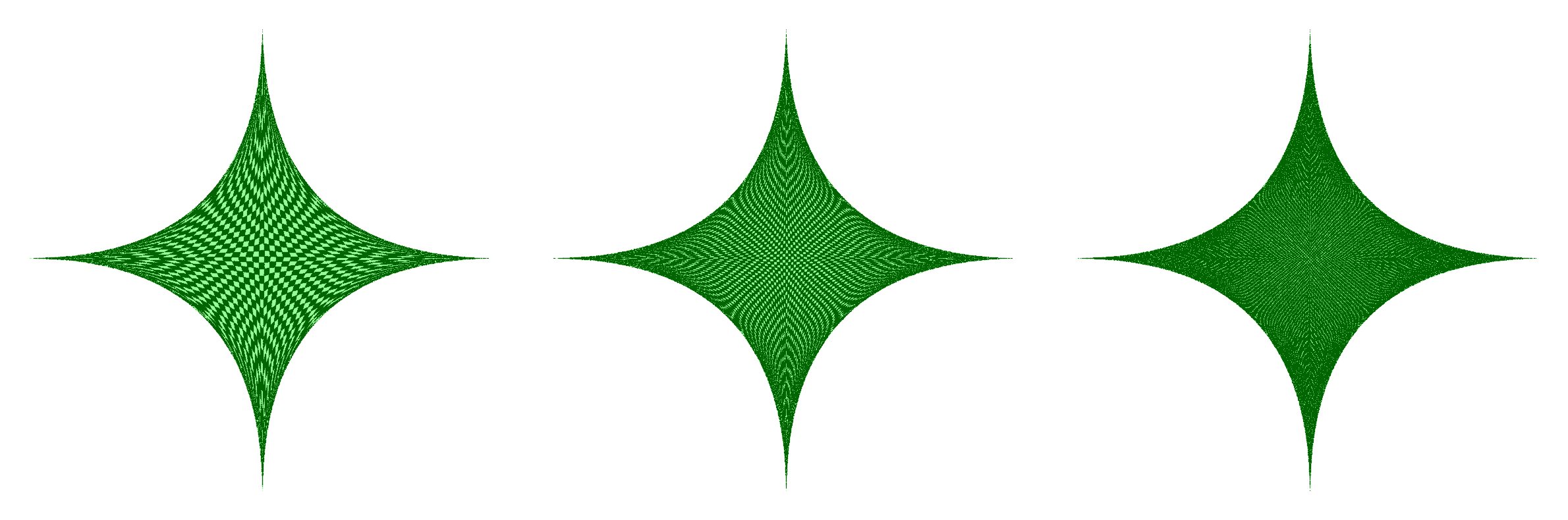
Example of gridification

🚀 How it works

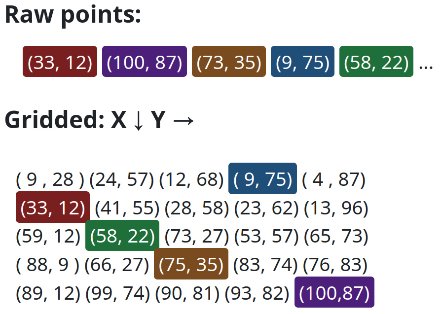
You initialize SquareNet with a target grid shape, then call fit() on your point cloud. Under the hood, the Cartesian sort algorithm rearranges point indices into structured grid multi-indices.

raw points      #(N, D)       →  sn.fit(X)        →  grid  #(N1, N2, ..., ND)
flat data       #(N, *C)      →  sn.map(X)        →  structured tensor  #(N1, ..., ND, *C)
structured tensor             →  sn.invert_map(X) →  back to flat view

The mapping is bijective, so invert_map is exact — no information lost.

⚙️ The Cartesian Sort Algorithm

General Optimal Transport (the theoretically correct solution to gridification) is O(N²) to O(N³) — intractable at scale. Cartesian sort is a fast heuristic that exploits the tensor structure of the grid to sidestep that complexity.

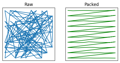
The idea is simple: loop over 1D Cartesian projections of the point cloud (x, y, z, …) and sort points along the corresponding grid axis (rows, columns, …). Each 1D sort is O(N log N) and fully vectorized. Since sorting along axis i+1 partially undoes the ordering along axis i, you repeat the full loop until all axes are sorted simultaneously — typically fewer than 50 iterations.

What you get:

Speed. ⏱️ Millions of points in seconds. All operations are native tensor ops.
Coordinate monotonicity. x increases along rows, y along columns, etc. This enable potential N-dimensional dychotomy principle for certain algorithms.
Approximate neighborhood preservation. Points close in space land close in the grid. Concrete experimental results on a 1M-point 2D dataset (France map, method='fast'):
- Requesting a 11×11 square window ([i-5:i+6, j-5:j+6] = 0.01% of candidates) → recovers ~97% of true nearest neighbors
- Requesting a 31×31 square window ([i-15:i+16, j-15:j+16] = 0.1% of candidates) → recovers ~99.5%
Volume conservation. Bijectivity naturally leads to conservation of volumes (or more generally measures: $\int \rho(x)\, dV$ when density rho is not constant in the point cloud). By conservation of volume, it is not mean that $\mathrm{vol}(g(A), g(B), g(C)) = \mathrm{vol}(A, B, C)$ where $ABC$ is a triangle, since the image of a triangle is generally not a triangle anymore. It would be equal to $\mathrm{vol}(\Omega),\qquad \Omega = \{ g(X) \mid X \in ABC \}$

What you don’t get:

Optimal Transport. SquareNet trades exactness for speed. If you need the provably optimal assignment, this isn’t the right tool.
Reverse neighborhood preservation. Close in space → close in grid, but not the other way around. Holes, clusters, and gaps in your data will be “closed” by the grid, which can place unrelated points next to each other.
Angular preservation. Volume and angles can’t both be conserved in the general case (classical result). Expect some distortion, especially near boundaries.

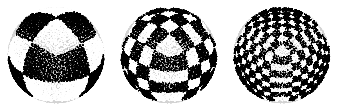
Three fitting modes

Mode	How it works	When to use
`fast` (default)	Raw Cartesian sort	General use, large datasets
`robust`	Sorts subgrids at each step	Less prone to local minima
`ultimate`	Adds random shearing perturbations	Near-zero outliers, but slow and require tuning `max_iter` parameter (bigger = better, but depending on scale and geometry sometimes 100 iterations are fine, sometimes best results require 10_000 iterations = 20 minutes fit for 1-M points dataset)

📦 Installation

pip install squarenet

🧠 Quick Start

→ See 00_getting_started.ipynb

from squarenet import SquareNet
import numpy as np

# 4D example: N points → 5×11×7×13 grid
N = 5 * 11 * 7 * 13
D = 4
X = np.random.rand(N, D)

sn = SquareNet(gridshape=(5, 11, 7, 13))
sn.fit(X)

# Inspect grid quality
sn.neighbormap()

# Map point data to grid and back
Xgrid = sn.map(X)         # shape (5, 11, 7, 13, D)
Xback = sn.invert_map(Xgrid)      # == X

Approximate nearest-neighbor search

point = np.random.rand(D)
index = sn.search_sorted(point)   # fast N-dimensional generalisation of  1D search sorted,
#will return a cell multi-index that best fit the given point (approximate method).

Index conversions

Working on a subset? mapidx converts flat point indices to grid multi-indices and back.

# Select points inside a disk, map their indices to the grid
sel = np.where(points[:, 0]**2 + points[:, 1]**2 <= 100) #raw indexes
gridsel = sn.mapidx(sel) #grid indexes
selback = sn.invert_mapidx(np.stack(gridsel, axis=1)) # == sel

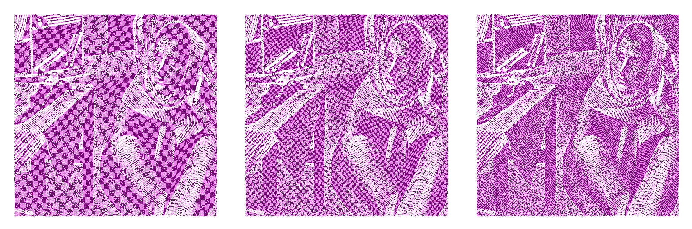
Visualizing the mapping

sn = SquareNet(gridshape=(400, 400))
sn.fit("france")
sn.plot()

📈 When to use SquareNet

Point cloud processing — fast spatial queries (neighbors, subsets) with contiguous memory lookup and vectorized tensorial processing instead of irregular kd-tree/voxels data structure
Kernel methods — efficient approximation of large Gram matrices via the grid structure
Deep learning — convert flat point datasets into tensors ready for CNNs or attention-based models

License: MIT

Author: ArmanddeCacqueray

Bijectivity requires that the product of the grid shapes equals N. If N is prime or not known in advance, pad your dataset with dummy points at ±∞ coordinates — they’ll land in the grid corners and won’t affect the rest of the mapping. ↩

This site is open source. Improve this page.